 arXiv
arXivControlling what a generative model produces usually means one of three things: fine-tune it on new data, attach a reward network that scores outputs, or run expensive search at inference time. All three are slow, brittle, or require labeled signal. This paper does something different: it steers a frozen model using only a handful of example images, exploiting a structural property of flow matching that makes this exact and efficient.
The idea
Guide with examples, not rewards.
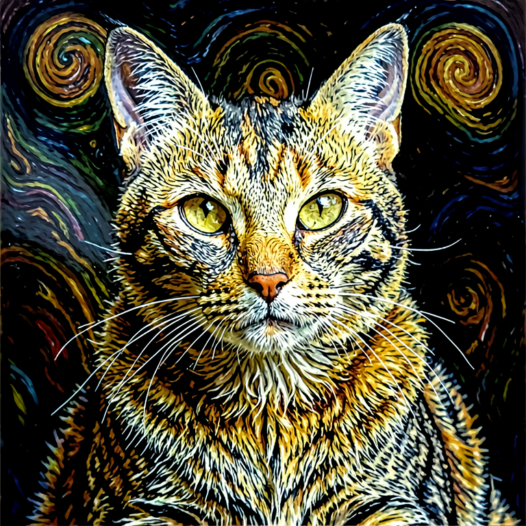
Think about how humans actually learn. Not by being scored on every move, but by watching someone do it first. You learn to cook by seeing a dish made. If you ask an artist to paint in the style of Van Gogh and hand them a reward signal at every brushstroke, they'll be lost. Show them a handful of Van Gogh paintings instead, and suddenly the task is clear — not because the examples are a perfect specification, but because they shift the artist's mental picture of where the painting should go.
The same intuition applies here, and flow matching makes it precise. At every step of generation, the model's velocity is entirely determined by one thing: where the model expects to end up — its conditional endpoint mean. That expectation is not a side product; it is the velocity. Shift the expectation, and the strokes change. Which means the examples aren't just intuition — they're the exact object you need to control.
And it turns out the math is simpler than you'd expect. Given a finite reference set, the reference endpoint mean has a closed form under a Gaussian bridge: a softmax-weighted sum over your reference images, where the weights are posterior probabilities computed from where you are in the trajectory. No neural network, no optimization loop. You compute it, apply a velocity correction proportional to the difference from the model's prediction, and you're done.
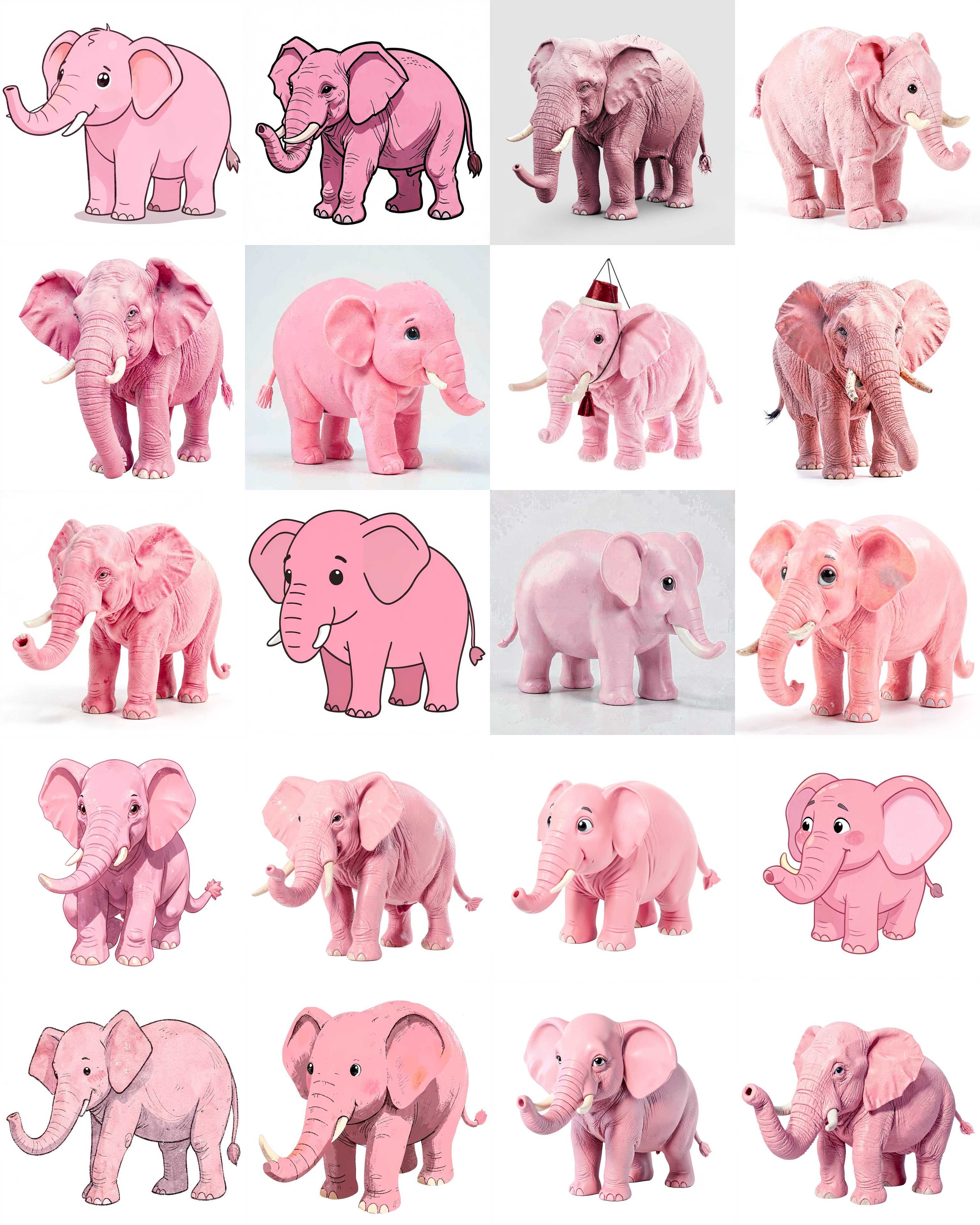
Best of all: the reference images don't need to match the prompt. They don't need to be high quality. They just need to encode the attribute you want to transfer. Twenty pink toy elephants will steer toward pink. Twenty Van Gogh paintings will steer toward impasto brushstrokes. The model never sees them during training. It sees them once, at inference time, and follows.
Method
How it works
The mechanism has three steps, each requiring only what the frozen model already computes.
01
Recover the endpoint mean
For any pretrained rectified-flow model, the endpoint mean is just μt(x) = x + (1 − t)ut(x). No extra computation needed: it falls out of the velocity prediction.
02
Compute a reference mean
Given M reference images, compute their posterior mean in closed form as a softmax-weighted sum. This is exact under a Gaussian bridge: the same math that underlies cross-attention.
03
Apply the correction
Add a scheduled velocity correction proportional to the difference between reference mean and model mean. No gradients, no backward pass, no auxiliary model.
Under the hood
The derivation
The three steps above have a clean derivation. This is where the endpoint-mean correction comes from, and why the reference mean takes the form of a softmax over examples.
Linear bridge
Same state
Expected velocity
Endpoint mean
Mean shift
Reference target
Guided mean
Guided velocity
Reference posterior
Attention form
Flow matching begins with a straight path from source noise to a data endpoint.
Many endpoint pairs can pass through the same intermediate point, so the flow averages over them. At inference time you don't know which endpoint you're heading toward — you only know where you are now. The marginal field has to be consistent with all possible endpoints that could have produced this state.
The marginal vector field is the conditional expectation of those bridge velocities.
For a Gaussian source, integrating out x0 leaves a velocity that depends on nothing except the expected endpoint — the model's running best guess of where the generation will land. This is the lever. Control the endpoint mean, and you control the flow.
You don't need to retrain anything, modify the architecture, or define a reward. To change where the model goes, you only need to shift one quantity: the conditional endpoint mean. The velocity correction falls out as a ratio — mean shift divided by time remaining. That's the entire mechanism.
We want a target distribution that interpolates between the model's prior and the reference density. A geometric mixture does this: β = 0 recovers the base model, β = 1 follows the reference entirely. This is an approximation — exact computation under the bridge is intractable — but under the Gaussian posterior assumption that holds in FLUX.2's VAE latent space, it gives the closed-form result that follows.
The geometric mixture produces a mean that is a convex combination of the model's prediction and the reference mean. βt is scheduled over the trajectory — usually near zero early, when structure is forming, and larger later, when details are resolved. You control how hard the references pull, and when.
Substituting that mean shift gives the practical correction used during sampling. The only missing ingredient is μ̂tρ, the approximate reference mean, which the next two steps compute from a finite bank of examples.
For a finite reference bank, the reference mean is a posterior-weighted average of examples. The weights αt(m) are posterior probabilities: how likely is each reference image to be the true endpoint, given where you are now in the trajectory? Under a Gaussian bridge, this posterior has a closed form. No inference network, no optimization.
The weights are a softmax over dot products between the current state xt and each reference image r(m), normalized by the bridge variance (1−t)2. This is cross-attention — not by analogy, but exactly. The current state is the query. The reference images are keys and values.
Part I
Reference-Mean Guidance
Training-free. Closed-form. Applied to a frozen 4B-parameter FLUX.2-klein model. The next three sections show what it does.
Reference-Mean Guidance · Results
Swap the reference set, change the output
Take the prompt "elephant in a jungle." A frozen FLUX.2-klein generates a reasonable image — grey elephant, green canopy. Now hand it twenty images of pink toy elephants. None of them contain jungles. None of them match the prompt. The prompt hasn't changed. The seed hasn't changed. The 4-billion model weights haven't changed. The output is now pink.
Swap the reference bank to blue elephants. The output turns blue.
That's the whole interface. A folder of images. Swappable at inference time, with no retraining. The nearest-neighbor column shows the closest image in the reference bank, so you can see that the model is being guided rather than simply copying.
The reference banks used below

Examples don't need to be perfect
Style change
Any reference set R that shifts the endpoint mean in the right direction works.
Examples don't need to be perfect
Attribute change
Any reference set R that shifts the endpoint mean in the right direction works.
Examples don't need to be perfect
Compositionality
Any reference set R that shifts the endpoint mean in the right direction works.

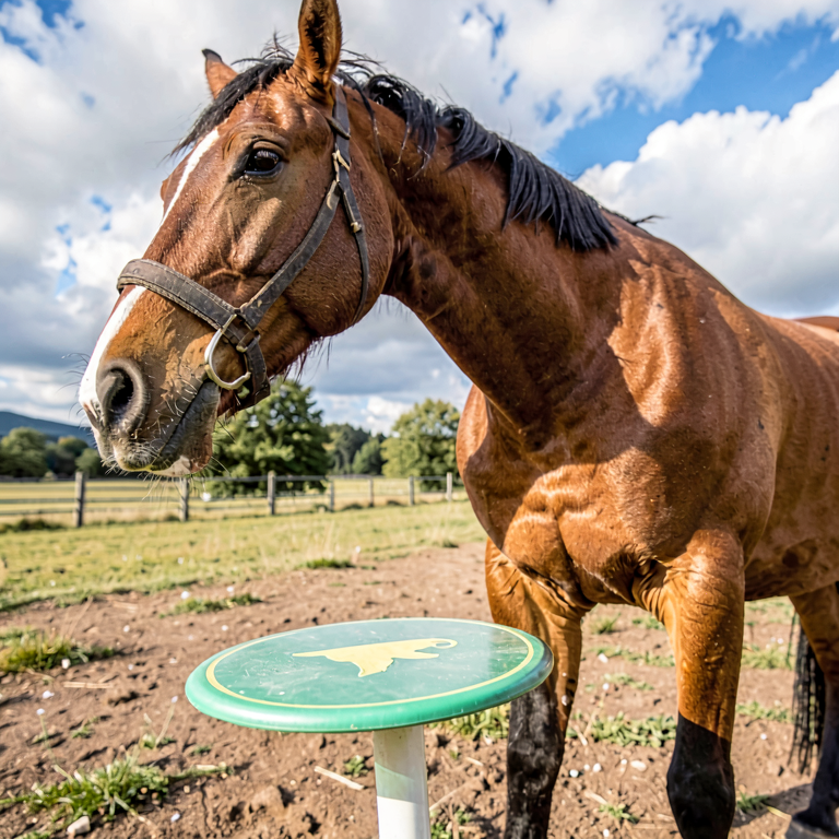
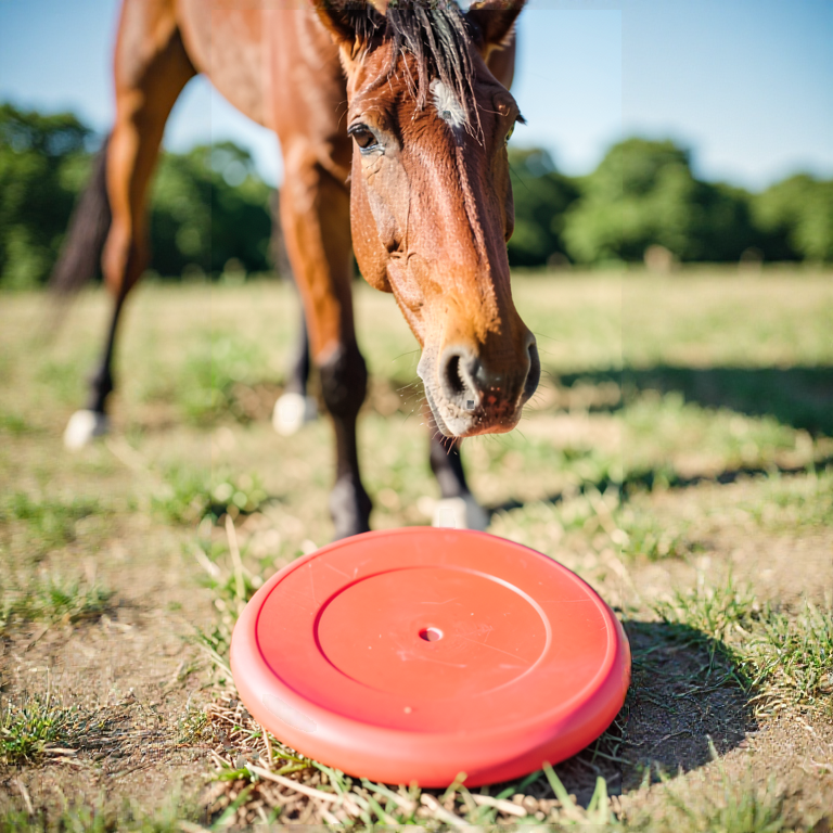
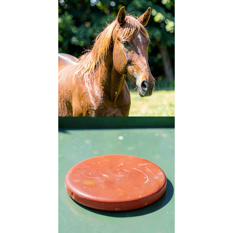
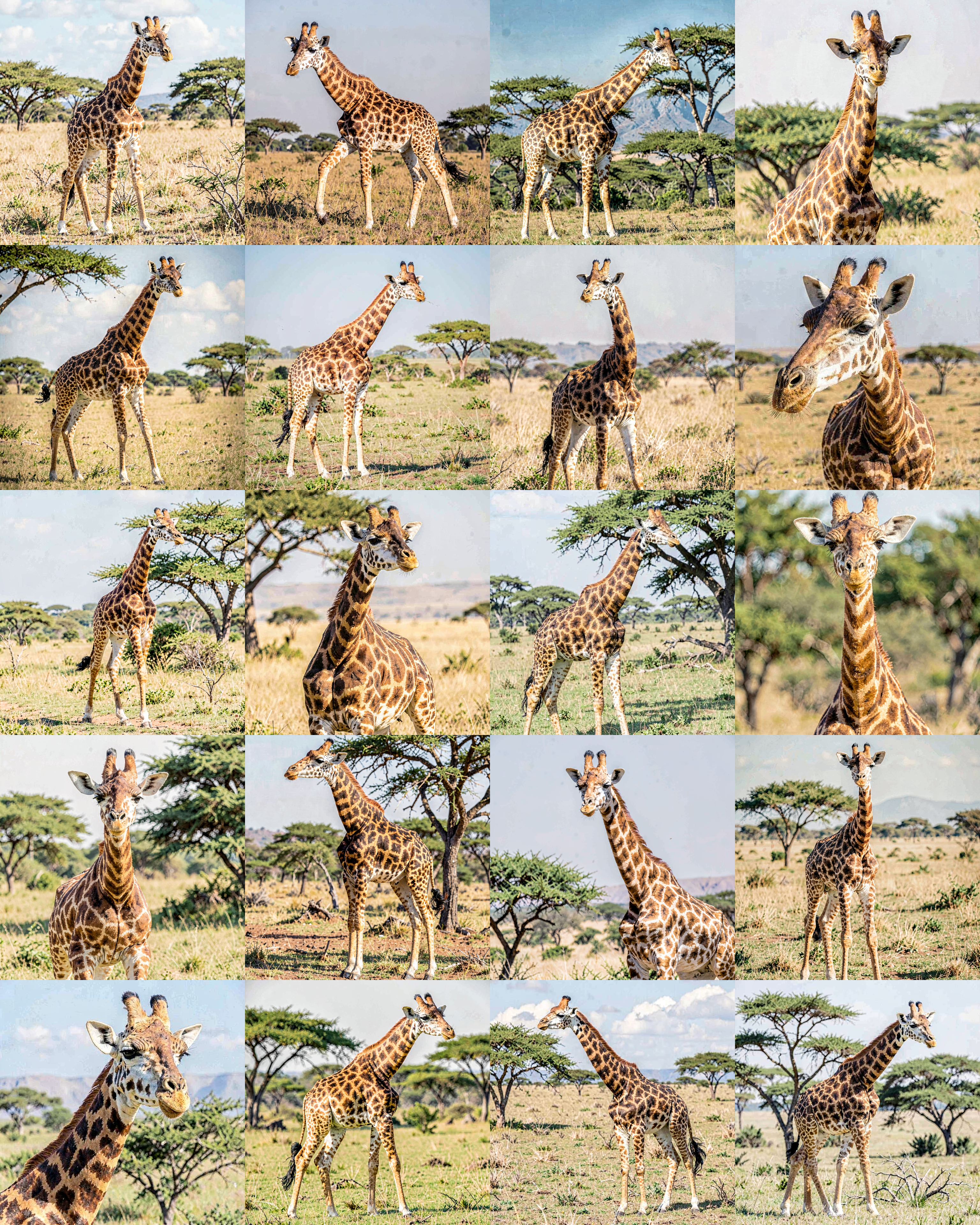
Structural control
It can even transfer geometry
We didn't expect this to work for structure.
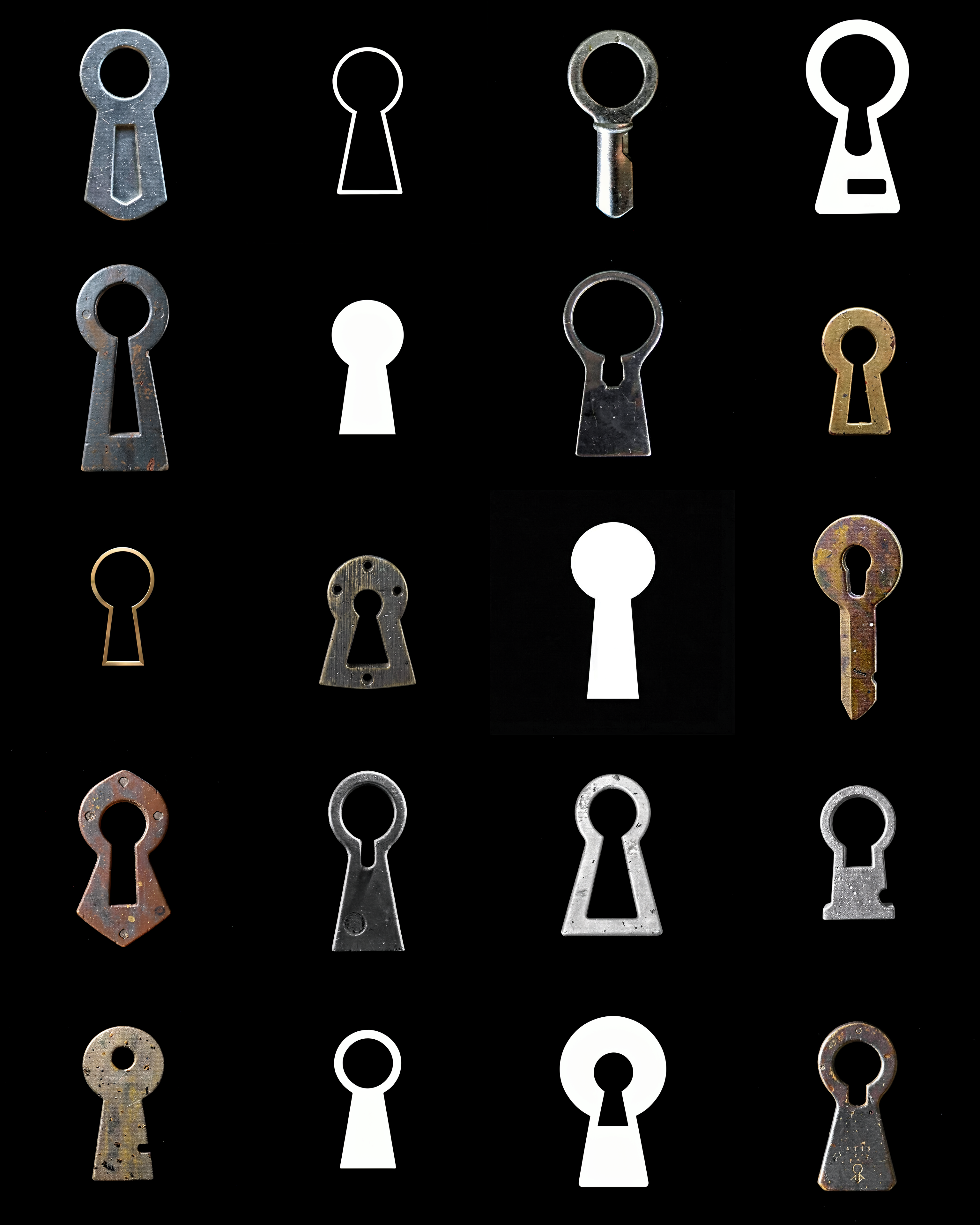
Structural correctness is hard to define as a reward: VLMs struggle to judge whether a hand is correctly oriented or a silhouette matches a target shape. Reference-mean guidance sidesteps this entirely: just show it examples of the target structure. No pose estimator, no spatial loss, no gradient.
Keyhole shape
a miniature forest...all inside a keyhole on a black background
Hand pose
a hand doing the sign of the horns
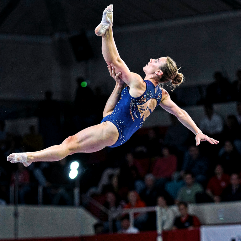
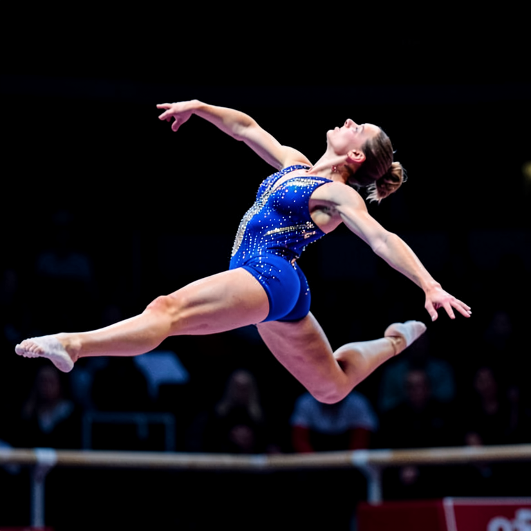
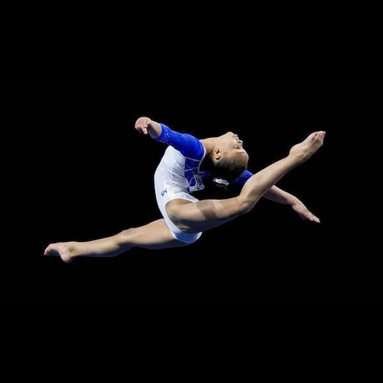
Gymnastics pose
a gymnast performing a ring leap...


GenEval benchmark
One forward pass. No reward model.
This comparison is between control interfaces, not a controlled ablation. RMG uses a fixed 20-image visual reference bank per category; baselines must express the same constraint through text prompts, classifier scores, or reward gradients. All methods share the same backbone, resolution, sampler, prompts, and seeds. The largest gains appear on compositional categories: position (+28.75) and two-object generation (+8.08), where text alone is insufficient to ground the target structure.
| Method | Time down | NFE down | Aux. down | Mean up | Two up | Position up | Attribution up |
|---|---|---|---|---|---|---|---|
| FLUX.2-klein (4B) baseline | 1.00x | 1x | - | 80.10 | 91.41 | 65.25 | 58.75 |
| Search-based | |||||||
| + Prompt Opt. | 7.87x | 8x | 8C+2L | 84.18 | 95.45 | 69.75 | 64.00 |
| + Best-of-4 | 4.07x | 4x | 4C | 83.35 | 95.96 | 67.75 | 65.25 |
| + SMC | 6.17x | 4x | 81C | 80.28 | 95.71 | 61.75 | 57.25 |
| Gradient-based | |||||||
| + ReNO | 19.44x | 4x | 4C | 83.46 | 93.18 | 65.50 | 64.75 |
| Ours (RMG) | 1.02x | 1x | - | 91.17 | 99.49 | 94.00 | 75.25 |
The largest gains are on the categories where text prompts consistently fail: position (+28.75 points) and two-object composition (+8.08). Showing the model examples of correct spatial arrangements works where describing them in text does not.
Semi-Parametric Guidance
A learned variant that knows what to copy
Reference-Mean Guidance has a limitation. The closed-form correction uses all of the reference bank's information — including things you don't want. A bank of pink toy elephants, all photographed against a white studio backdrop, will steer toward pink backgrounds as well as pink subjects. RMG can't distinguish between the attribute you care about and the ones that happen to correlate with it.
Semi-Parametric Guidance fixes this by amortizing the same idea into a learned architecture. Instead of applying the closed-form correction directly, SPG uses a cross-attention anchor to summarize the reference set, and a learned residual refiner to decide what to keep and what to suppress. The reference set is still swappable at inference time — nothing about that changes. But now the model can learn which aspects of the reference distribution are relevant to the generation task.
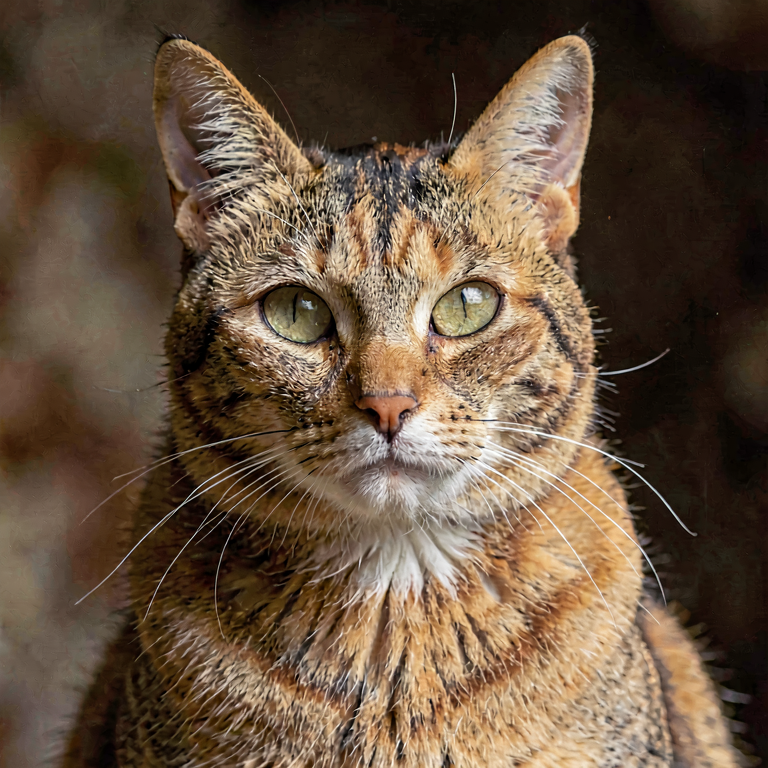
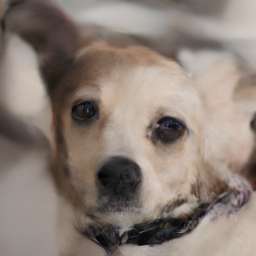
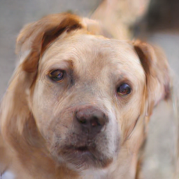
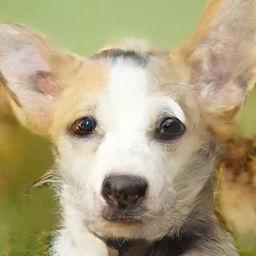
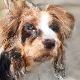
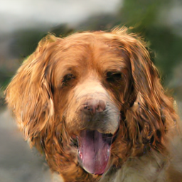
Trained on AFHQv2, SPG matches DiT-B/4 baseline quality (FID 23.26 vs 23.11), meaning the reference-set anchor doesn't degrade generation. And by swapping the reference set at inference time, you get continuous control over what the model generates: show it only cats, it generates cats; show it only dogs, it generates dogs; show it a mixture, it tracks the mixture proportions.
Unconditional generation quality on AFHQv2
| Method | FID down | KID down | IS up |
|---|---|---|---|
| DiT-B/4 baseline | 23.111 | 0.012 | 6.554 |
| SPG (ours) | 23.256 | 0.013 | 6.227 |
SPG matches DiT-B/4 baseline (FID 23.26 vs 23.11), confirming the reference-set anchor does not degrade generation quality.
Inference-time control
Generated class proportions closely track the reference-set composition across a wide range of reference sizes M, demonstrating continuous control without modifying model parameters.
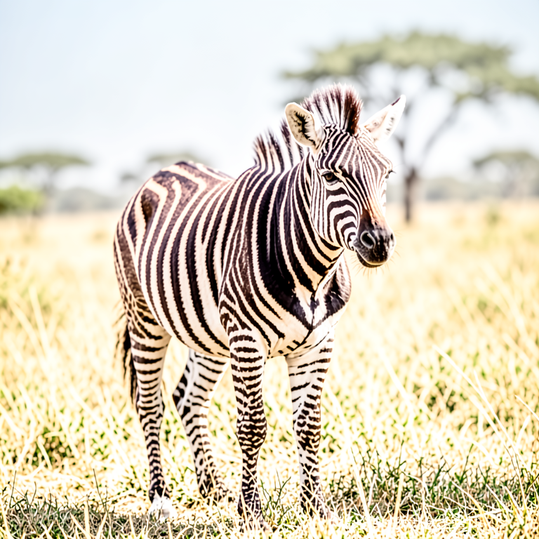
Reference-set swaps · same model, same noise
full reference set: generated
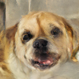
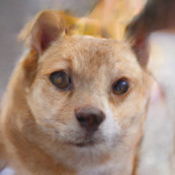
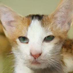
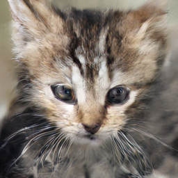
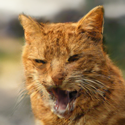
nearest neighbors (latent space): not copies
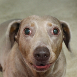
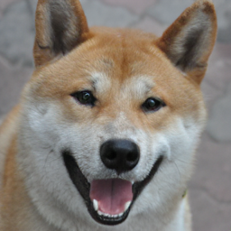
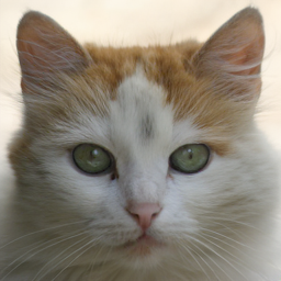
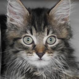
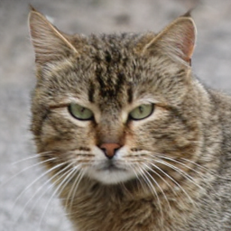
cat-only reference set
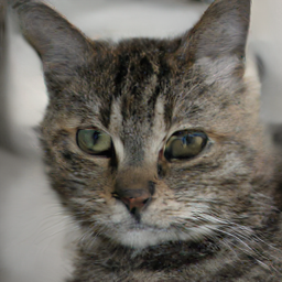
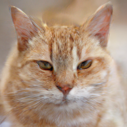
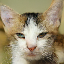
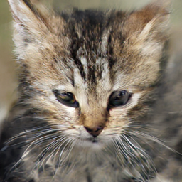
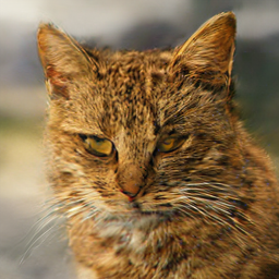
dog-only reference set
Conclusion
What this points toward
If control is represented by parameters, adaptation requires optimization and can create interference between concepts. If control is represented by a reference set, adaptation becomes a data operation: adding, removing, or reweighting examples changes the posterior mean and therefore the flow. This makes reference-guided flows naturally suited to low-data regimes, personalization, and continual adaptation settings where the target distribution changes faster than one would like to retrain a model.
Fine-tuning, reward networks, test-time search — these are the standard answers to controllable generation. Reference-guided flow matching suggests a different answer: a reference set. Swappable, interpretable, and requiring no gradient.
Citation
@misc{curvo2026followmeanreferenceguidedflow,
      title={Follow the Mean: Reference-Guided Flow Matching},
      author={Pedro M. P. Curvo and Maksim Zhdanov and Floor Eijkelboom and Jan-Willem van de Meent},
      year={2026},
      eprint={2605.10302},
      archivePrefix={arXiv},
      primaryClass={cs.LG},
      url={https://arxiv.org/abs/2605.10302},
}